いくつかのスナック菓子について食感の印象の評価を行い、スナック菓子の食感にどのような共通性があるかを、Rを使った因子分析で調べました。

評価から得られたデータはこんな感じ。

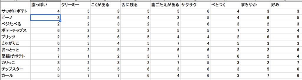
実際に全部食べて評価してます。笑

実は私の専攻では学部生向けに統計分析の実習があって、こんな感じで理論だけじゃなく実際にやってみて分析の流れを学ぶという素晴らしいものです。人気なので私のような院生も参加しちゃいます。せっかくなのでブログのネタに。

まず、上のデータをcsvで保存します。ちなみに、属性（ここでは評価の尺度）の数より刺激（スナック菓子）の数が多くなければ固有値分解ができないので注意です。

今回はRのpsychパッケージを利用して因子分析を行いました。いくつかライブラリをロードします。

library(psych) 
library(GPArotation) #因子軸の回転に使用します

次に、csvを読み込みます。ヘッダーを有効に、1列目をインデックスに指定してます。

data <- read.csv("okashi.csv", header = TRUE, row.names = 1, fileEncoding = "CP932")

因子数を決めます。MAP基準と平行分析を両方やってみて解釈します。

MAPminres <- vss(data, fm="minres") #MAP基準、最小残差法
print(MAPminres)

MAPml <- vss(data, fm="ml") #MAP基準、最尤法
print(MAPml)

parallel <- fa.parallel(data) #平行分析
print(parallel)

> MAPminres <- vss(data, fm="minres") #MAP基準、最小残差法
> print(MAPminres)

Very Simple Structure
Call: vss(x = data, fm = "minres")
VSS complexity 1 achieves a maximimum of 0.76  with  2  factors
VSS complexity 2 achieves a maximimum of 0.93  with  4  factors

The Velicer MAP achieves a minimum of 0.13  with  2  factors 
BIC achieves a minimum of  NA  with  1  factors
Sample Size adjusted BIC achieves a minimum of  NA  with  5  factors

Statistics by number of factors 
  vss1 vss2  map dof chisq  prob sqresid  fit RMSEA   BIC SABIC complex eChisq   SRMR eCRMS
1 0.75 0.00 0.19  27 40.94 0.042   6.189 0.75  0.42 -23.8  57.5     1.0 33.638 0.2061  0.24
2 0.76 0.90 0.13  19 22.45 0.262   2.385 0.90  0.38 -23.1  34.1     1.2  7.383 0.0966  0.13
3 0.69 0.92 0.19  12 14.04 0.298   1.455 0.94  0.43 -14.7  21.4     1.3  3.512 0.0666  0.12
4 0.71 0.93 0.28   6  9.11 0.167   0.574 0.98  0.58  -5.3  12.8     1.4  1.423 0.0424  0.10
5 0.69 0.88 0.33   1  4.27 0.039   0.104 1.00  1.19   1.9   4.9     1.5  0.108 0.0117  0.07
6 0.69 0.88 0.36  -3  2.45    NA   0.092 1.00    NA    NA    NA     1.5  0.092 0.0108    NA
7 0.69 0.88 0.50  -6  0.86    NA   0.049 1.00    NA    NA    NA     1.5  0.022 0.0053    NA
8 0.69 0.88 1.00  -8  0.46    NA   0.047 1.00    NA    NA    NA     1.5  0.020 0.0050    NA
   eBIC
1 -31.1
2 -38.2
3 -25.3
4 -13.0
5  -2.3
6    NA
7    NA
8    NA
> 
> MAPml <- vss(data, fm="ml") #MAP基準、最尤法
> print(MAPml)

Very Simple Structure
Call: vss(x = data, fm = "ml")
VSS complexity 1 achieves a maximimum of 0.74  with  2  factors
VSS complexity 2 achieves a maximimum of 0.94  with  4  factors

The Velicer MAP achieves a minimum of 0.13  with  2  factors 
BIC achieves a minimum of  NA  with  1  factors
Sample Size adjusted BIC achieves a minimum of  NA  with  5  factors

Statistics by number of factors 
  vss1 vss2  map dof   chisq  prob sqresid  fit RMSEA    BIC SABIC complex  eChisq    SRMR
1 0.72 0.00 0.19  27 37.6629 0.083 7.11958 0.72  0.39 -27.08  54.2     1.0 3.5e+01 2.1e-01
2 0.74 0.90 0.13  19 21.7763 0.296 2.57921 0.90  0.37 -23.78  33.4     1.3 7.1e+00 9.5e-02
3 0.69 0.92 0.19  12 14.0376 0.298 1.45482 0.94  0.43 -14.74  21.4     1.3 3.5e+00 6.7e-02
4 0.71 0.94 0.28   6  7.5484 0.273 0.55211 0.98  0.51  -6.84  11.2     1.4 1.6e+00 4.5e-02
5 0.69 0.88 0.33   1  3.1861 0.074 0.16976 0.99  1.01   0.79   3.8     1.5 2.3e-01 1.7e-02
6 0.69 0.88 0.36  -3  1.1720    NA 0.08266 1.00    NA     NA    NA     1.5 1.1e-01 1.2e-02
7 0.70 0.90 0.50  -6  0.1464    NA 0.01268 1.00    NA     NA    NA     1.5 1.0e-03 1.1e-03
8 0.69 0.88 1.00  -8  0.0056    NA 0.00022 1.00    NA     NA    NA     1.6 3.9e-06 7.1e-05
  eCRMS  eBIC
1  0.24 -29.5
2  0.13 -38.4
3  0.12 -25.3
4  0.11 -12.8
5  0.10  -2.2
6    NA    NA
7    NA    NA
8    NA    NA
> 
> parallel <- fa.parallel(data) #平行分析
Parallel analysis suggests that the number of factors =  2  and the number of components =  2

だいたい因子数が2つで説明できそうなので、因子数2で分析します。

nfactorsで因子数を指定。実際はデータに合わせて因子の抽出法も色々と検討すべきですが、とりあえずここではRでの分析方法の紹介ということで・・・。

res <- fa(data, nfactors=2, fm="minres", rotate="oblimin")
print(res, digits=3)

> res <- fa(data, nfactors=2, fm="minres", rotate="oblimin")
> print(res, digits=3)
Factor Analysis using method = minres
Call: fa(r = data, nfactors = 2, rotate = "oblimin", fm = "minres")
Standardized loadings (pattern matrix) based upon correlation matrix
 MR1 MR2 h2 u2 com
脂っぽい 0.073 0.997 0.964 0.0362 1.01
クリーミー 0.921 -0.109 0.908 0.0918 1.03
こくがある 0.808 -0.235 0.799 0.2006 1.17
舌に残る 0.902 0.323 0.779 0.2208 1.25
歯ごたえがある -0.536 0.415 0.566 0.4336 1.88
サクサク -0.038 -0.387 0.144 0.8561 1.02
べとつく -0.152 0.859 0.824 0.1762 1.06
まろやか 0.975 -0.010 0.955 0.0447 1.00
好み 0.163 -0.363 0.187 0.8130 1.39

 MR1 MR2
SS loadings 3.690 2.437
Proportion Var 0.410 0.271
Cumulative Var 0.410 0.681
Proportion Explained 0.602 0.398
Cumulative Proportion 0.602 1.000

 With factor correlations of 
 MR1 MR2
MR1 1.000 -0.239
MR2 -0.239 1.000

Mean item complexity = 1.2
Test of the hypothesis that 2 factors are sufficient.

The degrees of freedom for the null model are 36 and the objective function was 11.685 with Chi Square of 72.059
The degrees of freedom for the model are 19 and the objective function was 4.646 

The root mean square of the residuals (RMSR) is 0.097 
The df corrected root mean square of the residuals is 0.133 

The harmonic number of observations is 11 with the empirical chi square 7.383 with prob < 0.992 
The total number of observations was 11 with MLE Chi Square = 22.453 with prob < 0.262 

Tucker Lewis Index of factoring reliability = 0.6805
RMSEA index = 0.3801 and the 90 % confidence intervals are NA NA
BIC = -23.107
Fit based upon off diagonal values = 0.958
Measures of factor score adequacy 
 MR1 MR2
Correlation of scores with factors 0.996 0.994
Multiple R square of scores with factors 0.992 0.989
Minimum correlation of possible factor scores 0.984 0.978

バイプロットを作成。

biplot(res, labels=rownames(data))

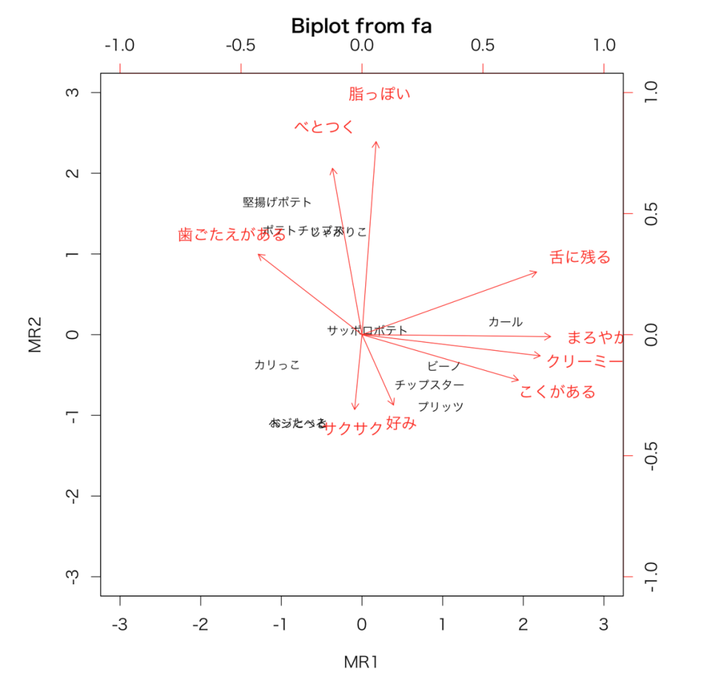
バイプロットを見ると、「舌に残る」、「まろやか」、「クリーミー」、「こくがある」が次元1に、「脂っぽい」、「べとつく」が次元2に対応しているかのような傾向が見れます。分析結果の寄与率（Proportion Var）が微妙なところですが、とりあえずしっちゃかめっちゃかな感じではなく傾向は出てる気がします。

このデータをどう解釈して因子をどう命名するかについては、色々あるのではしょりますが、こんな感じでとりあえずのところRで因子分析ができました。

ちなみにこんなデータも作ってみました。（実際お菓子のパッケージに表記されてるものから算出してますが、間違いがあるかもしれないのであしからず）

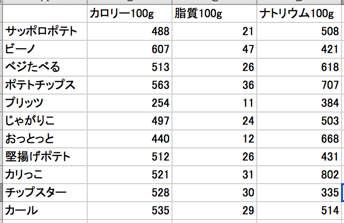
各次元との相関を見てみます。

cal <- read.csv("okashi_seibun.csv", header = TRUE, row.names = 1, fileEncoding = "CP932")

MR1_cal <- cor(res$scores[,1], cal[,1], method="spearman") #次元1とカロリーの相関
MR2_cal <- cor(res$scores[,2], cal[,1], method="spearman") #次元2とカロリーの相関
MR1_sisitsu <- cor(res$scores[,1], cal[,2], method="spearman") #次元1と脂質の相関
MR2_sisitsu <- cor(res$scores[,2], cal[,2], method="spearman") #次元2と脂質の相関
MR1_na <- cor(res$scores[,1], cal[,3], method="spearman") #次元1とナトリウムの相関
MR2_na <- cor(res$scores[,2], cal[,3], method="spearman") #次元2とナトリウムの相関

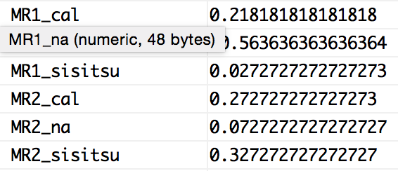
そんなにハッキリ出てはいないですが、「舌に残る」、「まろやか」、「クリーミー」、「こくがある」といった印象はナトリウムと逆の相関が見れます。「脂っぽい」、「べとつく」といった印象は、すこーし脂質と相関があるといった感じでしょうか。

私は最近健康志向だからか（笑）、「好み」の評価が次元2と逆に出ているのが面白いですね。